
When looking for an engagement ring for my (now) wife, the process involved first finding a suitable diamond that could be set into a ring of my choice. The process, which seems simple at first glance, became significantly more complex when presented with the numerous filtering options.

Which Attributes are Most Important?
In order to find the right diamond, you are presented with multiple options, such as:
| Carat: | Carat measures a diamond’s weight, not size. One carat equals 0.2 grams, and is divided into 100 points. For example, a 0.50ct diamond has 50 points. |
| Colour: | Colour grades range from D (colourless) to Z (noticeable yellow tint). The less colour, the more desirable and valuable the stone. |
| Clarity: | Clarity measures imperfections. VS2 or higher is considered ‘eye clean’. Imperfections are not visible without magnification. Scale: FL > IF > VVS1 > VVS2 > VS1 > VS2 > SI1 > SI2. |
| Cut: | Cut refers to how well a diamond reflects light. A better cut means more sparkle. Ranges include Fair, Good, Very Good, Excellent, and Cupid’s Ideal (‘hearts and arrows’ pattern). |
| Certificate: | The GIA is the most trusted certification body. Other labs like HRD and EGL can be less consistent, sometimes grading diamonds one to four grades differently than GIA. |
| Polish: | Polish assesses the smoothness of a diamond’s surface. High polish means fewer visible scratches or marks left after cutting. |
| Symmetry: | Symmetry refers to how evenly a diamond’s facets are placed. Better symmetry enhances brilliance and light return. Poor symmetry can reduce sparkle. |
| Fluorescence: | Fluorescence is a diamond’s reaction to UV light, often glowing blue. Strong fluorescence can make lower-colour diamonds appear whiter, but may cause haziness at high levels. Grades: None, Faint, Medium, Strong, Very Strong. |
| L/W Ratio: | Length-to-width ratio indicates how elongated a diamond appears when viewed from above. A round diamond has a ratio close to 1.0. Higher ratios indicate longer shapes. |
| Table: | The table is the diamond’s top flat facet. A balanced table size is key to optimal brilliance and light dispersion. |
| Depth: | Depth is the height from table to culet. Ideal depth (58–63%) allows for best light reflection. Too deep or shallow cuts reduce brilliance. |
Coupled with this non-exhaustive list of options, are the significant number of diamonds available for selection.
Just filtering on all diamonds over 0.3 carats, with the “Round” shape, gives us ~575,000 diamonds (as of July 2025).

I managed to find a fantastic diamond for my wife’s engagement ring seven years ago, but now with the prevalence of machine learning, I wondered if I could build a model to find me the right diamond if I had to select again.
Determining How to Extract the Data: Searching for an API
To build a model around the data, I needed to extract it for use. Given that there were 500k+ records, extracting this manually was not going to be feasible.
In addition to this, the webpage only allowed me to load 20 diamonds at a time. Given that there were 575,000 diamonds, this meant clicking this button 28,750 times!
I first tried to find if there was anyway to manipulate the number of results on the screen using the page URL, but all attempts failed:

For my next approach, I considered using a Python script with Selenium to automate clicking through the pop-ups (identified via their XPaths) and repeatedly trigger the “Load More Products” button, potentially up to 28,750 times; however, this proved unfeasible, as loading just 1,000 diamonds took nearly 20 minutes.
I needed a more systematic way to extract the data, so I started looking for an API, and after inspecting the calls made in the browser, I was quick to find this:
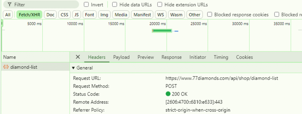
This was the API I was looking for, and I was able to grab the Payload to see which information was being sent to the API, and the Response to see the result that came back:
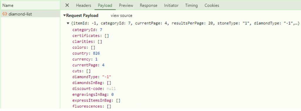
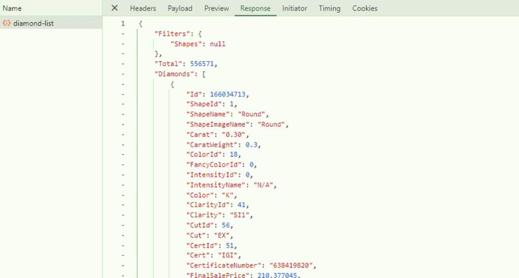
This gave me exactly what I needed!
Writing a Script to Pull Diamond Data
Now that I have a method to pull data via API, I wanted to write a simple Python script that would send the request, retrieve the response, and convert the data to a format that I could manipulate.
Using the “requests” package in Python, I attempted to run the API for all diamonds, but the request was quickly rejected.
Running the API for 500,000 results at once was not going to work, so the revised plan was to chunk the requests into smaller sizes. I settled on response sizes of 15,000 diamonds.
I was expecting around 40 responses from the API if I write the iterative function properly, but needed a way to ensure I had no duplicates across each of the extracts. In order to do this, I decided to use the “FinalSalePriceUSD” attribute, as the results returned were sorted by this attribute ascending (i.e. starts at hypothetical 0, and increases to the maximum price). If I find the maximum “FinalSalePriceUSD” in my extracted file, I could add a very small amount to it, and set it as the new minimum price in my next API extract.
To summarise, this is what I implemented:
- POST the request to the API where minPrice = 0 to retrieve the first 15,000 results, and save as “Response-1.json”
- Take the maximum value of the “FinalSalePriceUSD” attribute from “Response-1.json”
- POST the request to the API where minPrice = FinalSalePriceUSD + 0.0000001 (to avoid pulling duplicates) to retrieve an additional 15,000 results, and save as “Response-2.json”
- Repeat the process until all data has been extracted
First I initialised my script with the required packages, the API endpoint and headers and details of the payload. Next, I then take the returned reponse after successfully posting a payload (i.e. with a successful 200 status code), and then the JSON body is converted to a python dictionary for easier access:
import requests
import json
import os
import pandas as pd

os.makedirs('Extracts', exist_ok=True)

url = "https://www.77diamonds.com/api/shop/diamond-list"
headers = {
    "Content-Type": "application/json; charset=utf-8"
}

def call_api(min_price, page=1):
    payload = {
        "itemId": -1,
        "categoryId": 7,
        "currentPage": page,
        "resultsPerPage": 15000,
        "minPrice": min_price
    }
    response = requests.post(url, headers=headers, json=payload)
    return response.json()
To make sure I am able to define the “min_price” attribute based on the logic above (i.e. using the maximum “FinalSalePriceUSD” from the previous extract), I then define another function to determine this:
def get_max_final_sale_price(diamonds):
    if not diamonds:
        return None
    return max(d.get("FinalSalePriceUSD", 0) for d in diamonds)
Now that the functions are ready, I can write a Python script to iterative through the functions, to then pull each response and save them down in our “Extracts” folder:
min_price = 0
iteration = 1

while True:
    print(f"Fetching chunk {iteration} with minPrice = {min_price}")
    data = call_api(min_price)

    diamonds = data.get("Diamonds", [])
    total = data.get("Total", 0)
    status = data.get("Status", "Unknown")

    print(f"Status: {status}")
    print(f"Diamonds returned this chunk: {len(diamonds)}")
    print(f"Total matching diamonds: {total}")

    if not diamonds:
        print("No more diamonds retrieved. Exiting.")
        break

    filename = f"Extracts/Response-{iteration}.json"
    with open(filename, "w") as f:
        json.dump(data, f, indent=2)
    print(f"Saved {len(diamonds)} diamonds to {filename}")

    max_price = get_max_final_sale_price(diamonds)
    if max_price is None:
        print("No valid max price found. Exiting.")
        break

    next_min_price = max_price + 0.000001
    if next_min_price <= min_price:
        print("No progress in minPrice. Exiting.")
        break

    min_price = next_min_price
    iteration += 1
Dealing with Datatypes
Once all of the Response JSONs were in place, I then wanted to convert them to Parquet as the file sizes would be more manageable, and I could load this format easily into a Pandas dataframe.
One of the biggest challenges I faced initially, was that after I converted to Parquet, the data type of one attribute in one file didn’t necessarily match the data type of the same attribute in another. When I attempted to concatenate the files, this created issues.
To get around this, I just created a “forced_dtypes” dictionary, that I could use when converting each JSON to Parquet, ensuring that the dtypes were consistent:
import pyarrow
import os
import json
import pandas as pd

# Define the expected dtypes per field - need this as each parquet file decides what dtype it wants
# and its not necessarily the same across files
forced_dtypes = {
    "Id": "Int64",
    "ShapeId": "Int64",
    "ShapeName": str,
    "ShapeImageName": str,
    "Carat": float,
    "CaratWeight": float,
    "ColorId": "Int64",
    "FancyColorId": "Int64",
    "IntensityId": "Int64",
    "IntensityName": str,
    "Color": str,
    "ClarityId": "Int64",
    "Clarity": str,
    "CutId": "Int64",
    "Cut": str,
    "CertId": "Int64",
    "Cert": str,
    "CertificateNumber": "Int64",
    "FinalSalePrice": float,
    "FinalSalePriceGBP": float,
    "FinalSalePriceIncVATFloat": float,
    "FinalSalePriceIncVAT": float,
    "FinalCostPrice": float,
    "FinalCostPriceForWL": float,
    "FinalExVatCostPriceForWL": float,
    "FinalSalePriceUSD": float,
    "CurrencyCode": str,
    "Price": float,
    "Ratio": float,
    "Lw": float,
    "Code": str,
    "DepthPercent": "Int64",
    "TablePercent": "Int64",
    "PolishId": "Int64",
    "Polish": str,
    "SymmetryId": "Int64",
    "Symmetry": str,
    "FluorescenceId": "Int64",
    "Flo": str,
    "Depth": float,
    "Width": float,
    "Length": float,
    "Measurements": str,
    "WebMeasurements": str,
    "CuletId": "Int64",
    "Culet": str,
    "ImageUrl": str,
    "ActualPhotoUrl": str,
    "PhotoWidth": "Int64",
    "PhotoHeight": "Int64",
    "OtherCode": str,
    "PairedCode": str,
    "ETA": "Int64",
    "SupplierId": "Int64",
    "PairedWithCode": str,
    "StockNumber": str,
    "WLCode": str,
    "Light": str,
    "DiscountPercent": "Int64",
    "HasVideo": bool,
    "HasImage": bool,
    "IsFancy": bool,
    "ShowCertificate": bool,
    "CertificateUrl": str,
    "CountryOfOrigin": str,
    "IsSold": bool,
    "QuickShipping": bool,
    "DispatchDate": "datetime64[ns]",
    "DeliveryDate": "datetime64[ns]",
    "DiamondPrice": float,
    "AggregatedSupplierID": "Int64",
    "HiddenAttributes": str,
    "StoneTypeID": "Int64",
    "GemColorID": "Int64",
    "GemIntensityID": "Int64",
    "GemTreatmentID": "Int64",
    "GemClarityTreatmentID": "Int64",
    "GemTypeID": "Int64",
    "GemClarityID": "Int64",
    "CountryOfOriginId": "Int64",
    "StoneTypeAttributeId": "Int64",
    "StoneTypeName": str,
    "GemColorName": str,
    "GemIntensityName": str,
    "GemTreatmentName": str,
    "GemTypeName": str,
    "GemClarityName": str,
    "GemClarityTreatmentName": str
}

input_folder = "Extracts"
output_folder = "Parquet"
os.makedirs(output_folder, exist_ok=True)

for filename in os.listdir(input_folder):
    if filename.endswith(".json"):
        json_path = os.path.join(input_folder, filename)
        with open(json_path, "r", encoding="utf-8") as f:
            data = json.load(f)

        diamonds = data.get("Diamonds", [])
        if not diamonds:
            print(f"{filename} has no diamonds.")
            continue

        df = pd.DataFrame(diamonds)

        # Enforce dtypes - needed in particular for datetime which doesn't work by default above
        for col, dtype in forced_dtypes.items():
            if col in df.columns:
                if dtype == "datetime64[ns]":
                    df[col] = pd.to_datetime(df[col], errors="coerce")
                else:
                    df[col] = df[col].astype(dtype, errors="ignore")

        # Write each response to Parquet
        parquet_name = filename.replace(".json", ".parquet")
        parquet_path = os.path.join(output_folder, parquet_name)
        df.to_parquet(parquet_path, engine="pyarrow", index=False)
        print(f"Saved: {parquet_path}")
Finally, I can combine each of the files together into a master dataset ready for my training model:
from pathlib import Path

# Folder where the converted parquet files sit, as will need to pick them up
# to create the combined file
input_folder = Path("Parquet")
output_file = "combined_output.parquet"

parquet_files = sorted(input_folder.glob("*.parquet"))

# Load each file, and then concatenate them together into a combined_df
df_list = [pd.read_parquet(f) for f in parquet_files]
combined_df = pd.concat(df_list, ignore_index=True)

# Drop duplicates just incase any diamonds with the same ID appear more than once
# (though this should be managed with the maxPrice function above)
combined_df = combined_df.drop_duplicates(subset="Id")

# Write the combined DataFrame to a new parquet file
combined_df.to_parquet(output_file, engine="pyarrow", index=False)

print(f"Combined {len(parquet_files)} files into {output_file} with {len(combined_df):,} rows.")
Training my Price Prediction Models
Ridge Regression: Prediction with Log Prices
To start, I took the data I extracted via API, and limited the number of attributes that I wanted to run the model on, with the most common features chosen by prospective buyers those that I retained.
Many of the attributes were not numerical in value, so I needed to create dummy variables to represent qualitative features (e.g. Certification has values of IGI, GIA, etc. – I create a dummy variable for IGI and GIA that are 0 or 1 depending on the certificate for the particular diamond).
import pandas as pd
import numpy as np
import seaborn as sns
from sklearn.model_selection import train_test_split
from sklearn.preprocessing import StandardScaler
from sklearn.linear_model import Ridge
from sklearn.metrics import mean_squared_error, r2_score
import matplotlib.pyplot as plt

# Define the Parquet file path - using r' before the location tells python
# to treat backslashes as literal characters
parquet_file = r'C:\Users\Laith\Desktop\Python Projects\Diamond ML Model\combined_output.parquet'

# Read the Parquet file into a DataFrame
df = pd.read_parquet(parquet_file, engine='pyarrow')

primary_columns = [
    'Code','Carat','Color','Clarity','Cut','Cert','Polish','Symmetry',
    'Flo','Lw','TablePercent','DepthPercent','FinalSalePriceGBP']

primary_df = df[primary_columns]

intermediate_df = pd.get_dummies(primary_df,
                                 columns=['Color','Clarity','Cut','Cert','Polish','Symmetry','Flo'],
                                 drop_first=False)
For my first attempt at building a model, my immediate thought was to run a multifactor regression, with the Final Sale Price as the dependent variable, that would be explained by the values in my multiple independent variables.
Given the relatively simple start to this process, I prioritised the use of the Ridge Regression, for the following reasons:
- It is preferred over Linear Regression as doesn’t place too much trust in any one variable – this reduces the likelihood of “overfitting”, by reducing the coefficient size of certain variables,
- The Regression model handles multicollinearity well – in other words, if two features are very similar, the coefficient is shared between them, rather than given to just one attribute,
- Due to the number of dummy variables I created, Ridge Regression handles this well, as it balances them fairly, rather than allowing one to dominate,
- It’s a really good starting point, before considering more complex models such as XGBoost and Random Forest.
In essence, it is minimising the usual sum of squared errors as with Linear Regression, but includes a penalty term:
Despite these benefits, Ridge Regression is a still a linear model, and with my limited knowledge of diamonds, I knew that as the carat of the diamond increased, the price didn’t rise linearly (more like exponentially!)
A 1 carat diamond could cost £5,000, but that didn’t mean a 10 carat diamond would cost £50,000 – it almost certainly would be a lot higher than this.
In order to correct for this, and allow my (linear) Ridge Regression approach to hopefully work, I took the log value of the Final Sale Price, as the new dependent variable.
if 'LogFinalSalePriceGBP' not in intermediate_df.columns:
    intermediate_df['LogFinalSalePriceGBP'] = np.log(intermediate_df['FinalSalePriceGBP'])

X_full = intermediate_df.drop(columns=['LogFinalSalePriceGBP', 'FinalSalePriceGBP', 'Code'])
y_full = intermediate_df['LogFinalSalePriceGBP']

# Split
X_train, X_test, y_train, y_test = train_test_split(X_full, y_full, test_size=0.2, random_state=42)

# Scale
scaler = StandardScaler()
X_train_scaled = scaler.fit_transform(X_train)
X_test_scaled = scaler.transform(X_test)

# Train Ridge
ridge = Ridge(alpha=1, solver='svd')
ridge.fit(X_train_scaled, y_train)

# Evaluate
y_pred_test = ridge.predict(X_test_scaled)
print("R²:", r2_score(y_test, y_pred_test))
print("MSE:", mean_squared_error(y_test, y_pred_test))
The outcome of the model was to return a very good R-squared value of 0.7982 and Mean Squared Error of 0.2009 – this was promising.
Now that I have a model that looks to have a great predictive power, I wanted to run through a hypothetical scenario to see whether I could find “underpriced” diamonds for my selected options, relative to the predicted price.
Now that I have my model in place, I wanted to run through a hypothetical scenario of my ideal diamond with the following characteristics:
- The number of Carats needs to be between 1 and 2
- I want either an Excellent or Very Good Polish
- The diamond needs to have a Flawless Quality
- The Colour of the diamond needs to be the highest classification (i.e. D – the whitest)
My ideal diamond will be the one where the Predicted Price – Actual Price is maximised in relative terms.
I create a quick script to run through this scenario:
# Create a copy of my ideal diamonds and store in a new variable
ideal_df = intermediate_df[intermediate_df['IsIdeal'] == 1].copy()

# Prepare features
X_premium = ideal_df.drop(columns=['LogFinalSalePriceGBP', 'FinalSalePriceGBP', 'Code', 'IsIdeal'])
X_premium_scaled = scaler.transform(X_premium)

# Predict
log_preds = ridge.predict(X_premium_scaled)
ideal_df['PredictedPrice'] = np.exp(log_preds)
ideal_df['UnderpricingAmount'] = ideal_df['FinalSalePriceGBP'] - ideal_df['PredictedPrice']
ideal_df['UnderpricingPct'] = ideal_df['UnderpricingAmount'] / ideal_df['PredictedPrice']

# Find most underpriced
most_underpriced = ideal_df.sort_values(by='UnderpricingAmount').head(1).squeeze()

print("\n💎 Most Underpriced Diamond (Model thinks it should cost more):")
print(f"🔹 Code: {most_underpriced['Code']}")
print(f"🔹 Carat: {most_underpriced['Carat']:.2f}")
print(f"🔹 Final Sale Price (GBP): £{most_underpriced['FinalSalePriceGBP']:,.2f}")
print(f"🔹 Predicted Price (GBP): £{most_underpriced['PredictedPrice']:,.2f}")
print(f"🔹 Underpricing Amount: £{most_underpriced['UnderpricingAmount']:,.2f}")
print(f"🔹 Underpricing %: {most_underpriced['UnderpricingPct']:.2%}")
💎 Most Underpriced Diamond (Model thinks it should cost more):
🔹 Code: RBPUIFS8HCDHCU7
🔹 Carat: 1.13
🔹 Final Sale Price (GBP): £8,337.42
🔹 Predicted Price (GBP): £5,039.61
🔹 Underpricing Amount: £3,297.81
🔹 Underpricing %: 65.44%
The results are a little disappointing… the model is suggesting that the best value of money diamond has an actual price of £8,337.42, but my predicted price is £5,039.61. Something is going wrong.
I checked the full set of ~150 diamonds with the ideal characteristics, and indeed found that the selected diamond was the “best priced” based on my model, but every single diamond in this range was predicting a price far lower than the actual prices.
When investigating, I came to the following conclusions:
- My dataset was heavily skewed towards lower priced diamonds – a majority of the data was bucnhed up at the lower end of the price range
- My ideal diamond was looking for a combination of highly sought after and rare combinations of Clarity and Colour – a model trained on many diamonds not in the range failed to capture the premium
Ridge Regression: Inclusion of “Price per Carat”
In order to correct for this, I looked into previous models built around this data, and found that it was very common to incorporate a “Price-per-Carat” divisor – I would effectively divide the FinalSalePrice by the Carat to get a “Price-per-Carat” value that I could then test my model on.
intermediate_df = intermediate_df[intermediate_df['Carat'] > 0].copy()

intermediate_df['PricePerCarat'] = intermediate_df['FinalSalePriceGBP'] / intermediate_df['Carat']
intermediate_df['LogPricePerCarat'] = np.log(intermediate_df['PricePerCarat'])

# Drop irrelevant columns
X = intermediate_df.drop(columns=[
    'FinalSalePriceGBP', 'PricePerCarat', 'LogPricePerCarat', 'Code'
])
y = intermediate_df['LogPricePerCarat']

# Train/test split
X_train, X_test, y_train, y_test = train_test_split(X, y, test_size=0.2, random_state=42)

# Standardise
scaler = StandardScaler()
X_train_scaled = scaler.fit_transform(X_train)
X_test_scaled = scaler.transform(X_test)

# Train model
model = Ridge(alpha=1.0)
model.fit(X_train_scaled, y_train)

# Evaluate
y_pred_test = model.predict(X_test_scaled)
print("R²:", r2_score(y_test, y_pred_test))
print("MSE:", mean_squared_error(y_test, y_pred_test))
This time, the model returns a far better R-squared value and Mean Squared Error (0.9485 & 0.0157), so I am hoping that this will have better predictive power for my particular selection.
Using the same classification of my ideal diamond as above, I run the model again:
# Filtered FL-D diamonds
filtered_df = intermediate_df[
    (intermediate_df['Carat'] >= 1) & (intermediate_df['Carat'] <= 2) &
    ((intermediate_df['Polish_VG'] == 1) | (intermediate_df['Polish_EX'] == 1)) &
    (intermediate_df['Clarity_FL'] == 1) &
    (intermediate_df['Color_D'] == 1)
].copy()

# Predict
X_filtered = filtered_df.drop(columns=[
    'FinalSalePriceGBP', 'PricePerCarat', 'LogPricePerCarat', 'Code'
])
X_filtered_scaled = scaler.transform(X_filtered)

filtered_df['PredictedLogPPC'] = model.predict(X_filtered_scaled)
filtered_df['PredictedPPC'] = np.exp(filtered_df['PredictedLogPPC'])
filtered_df['PredictedPrice'] = filtered_df['PredictedPPC'] * filtered_df['Carat']

# Now calculate predicted price
filtered_df['PredictedPrice'] = filtered_df['PredictedPPC'] * filtered_df['Carat']

# Underpricing calc
filtered_df['UnderpricingAmount'] = filtered_df['FinalSalePriceGBP'] - filtered_df['PredictedPrice']
filtered_df['UnderpricingPct'] = filtered_df['UnderpricingAmount'] / filtered_df['PredictedPrice']

# Show the most underpriced one (most negative UnderpricingAmount)
most_underpriced = filtered_df.sort_values(by='UnderpricingAmount').head(1).squeeze()

print("\n💎 Most Underpriced Diamond (Model thinks it should cost more):")
print(f"🔹 Code: {most_underpriced['Code']}")
print(f"🔹 Carat: {most_underpriced['Carat']:.2f}")
print(f"🔹 Final Sale Price (GBP): £{most_underpriced['FinalSalePriceGBP']:,.2f}")
print(f"🔹 Predicted Price (GBP): £{most_underpriced['PredictedPrice']:,.2f}")
print(f"🔹 Underpricing Amount: £{most_underpriced['UnderpricingAmount']:,.2f}")
print(f"🔹 Underpricing %: {most_underpriced['UnderpricingPct']:.2%}")
💎 Most Underpriced Diamond (Model thinks it should cost more):
🔹 Code: RBILNBXVFSJD
🔹 Carat: 1.67
🔹 Final Sale Price (GBP): £20,203.61
🔹 Predicted Price (GBP): £22,738.89
🔹 Underpricing Amount: £-2,535.28
🔹 Underpricing %: -11.15%
The results are much better – the diamond identified by the model as the best value for money gives one with a Final Sale Price almost £2,500 less than the Predicted Price:

To satisfy my curiosity, I want to try two other models to see if I can increase the accuracy further.
XGBoost: Assessing Decision Trees
XGBoost stands for eXtreme Gradient Boosting, and is a Machine Learning model that starts by building a decision tree to predict the value of the dependent variable (in this case, the Final Sale Price), and then tries to improve on this prediction by making small improvements to the next decision tree to minimise the sum of squared error.
In terms of my diamonds data, the process could look something like:
- The first decision tree is produced, that predicts a price of £5,000
- It then is compared against the actual price of £6,000, to determine the error as £1,000
- The next tree is then trained to predict the same error (the residual)
- The correction from the second tree is added to the first prediction
- The process repeats to continue minimising the sum of squared errors – if the error keeps reducing, the model continues, else it stops
In terms of the maths, the intention is to minimise the following function (which in layman’s terms is Loss (how far off the prediction was) + Regularisation (the penalty applied for complexity)):
The point of XGBoost, is to reduce the Loss part of the function (as a smaller value means the predicted price is closer to the actual price), while also trying to reduce the addition for regularisation (where the value increases as a penalty in proportion to the model complexity).
XGBoost is quite popular online, having been a staple of Kaggle competitions for its fast predictions, high accuracy and ability to avoid the overfitting issue I experienced with the initial Ridge Regression I performed.
from xgboost import XGBRegressor
from sklearn.model_selection import train_test_split
from sklearn.metrics import r2_score, mean_squared_error

# Features and target
X = intermediate_df.drop(columns=['LogFinalSalePriceGBP', 'FinalSalePriceGBP', 'Code', 'IsIdeal'])
y = intermediate_df['LogFinalSalePriceGBP']

# Train/test split
X_train, X_test, y_train, y_test = train_test_split(X, y, test_size=0.2, random_state=42)

# Train XGBoost model
xgb = XGBRegressor(n_estimators=100, learning_rate=0.1, max_depth=4, random_state=42)
xgb.fit(X_train, y_train)

# Evaluate
y_pred_xgb = xgb.predict(X_test)
print("XGBoost R²:", r2_score(y_test, y_pred_xgb))
print("XGBoost MSE:", mean_squared_error(y_test, y_pred_xgb))
This model has given me the best R-squared value and Mean Squared Error yet (0.9991 & 0.0009).
Now using the model, it will be interesting to see whether the “best priced” diamond based on the model price predictions has a larger relative difference than the Ridge Regression or not:
# Filter ideal diamonds
ideal_xgb_df = intermediate_df[intermediate_df['IsIdeal'] == 1].copy()

# Drop unneeded columns
X_ideal_xgb = ideal_xgb_df.drop(columns=['LogFinalSalePriceGBP', 'FinalSalePriceGBP', 'Code', 'IsIdeal'])

# Predict log prices
log_preds_xgb = xgb.predict(X_ideal_xgb)

# Convert back from log
ideal_xgb_df['PredictedPrice_XGB'] = np.exp(log_preds_xgb)

# Calculate difference
ideal_xgb_df['Underpricing_XGB'] = ideal_xgb_df['FinalSalePriceGBP'] - ideal_xgb_df['PredictedPrice_XGB']

# Underpricing calc
ideal_xgb_df['UnderpricingAmount'] = ideal_xgb_df['FinalSalePriceGBP'] - ideal_xgb_df['PredictedPrice_XGB']
ideal_xgb_df['UnderpricingPct'] = ideal_xgb_df['Underpricing_XGB'] / ideal_xgb_df['PredictedPrice_XGB']

# Show the most underpriced one (most negative UnderpricingAmount)
most_underpriced = ideal_xgb_df.sort_values(by='UnderpricingAmount').head(1).squeeze()

print("\n💎 Most Underpriced Diamond (Model thinks it should cost more):")
print(f"🔹 Code: {most_underpriced['Code']}")
print(f"🔹 Carat: {most_underpriced['Carat']:.2f}")
print(f"🔹 Final Sale Price (GBP): £{most_underpriced['FinalSalePriceGBP']:,.2f}")
print(f"🔹 Predicted Price (GBP): £{most_underpriced['PredictedPrice_XGB']:,.2f}")
print(f"🔹 Underpricing Amount: £{most_underpriced['UnderpricingAmount']:,.2f}")
print(f"🔹 Underpricing %: {most_underpriced['UnderpricingPct']:.2%}")
💎 Most Underpriced Diamond (Model thinks it should cost more):
🔹 Code: RBCPGFTQEBYR
🔹 Carat: 1.72
🔹 Final Sale Price (GBP): £21,869.46
🔹 Predicted Price (GBP): £23,471.55
🔹 Underpricing Amount: £-1,602.09
🔹 Underpricing %: -6.83%
The model is finding a diamond with an underpricing of a smaller margin than the Ridge Regression. The fact that the R-squared value and Mean Squared Error were far more favourable, means I am more likely to trust that this model is a better predictor of what a diamond price should be.
Now I want to try one final model – the Random Forest.
Random Forest: Building a Decision Tree Forest
Random Forest is a Machine Learning algorithm that builds a “forest” of multiple decision trees, and combines them to improve predictions (as opposed to improving on one over and over).
It has a similar benefit to XGBoost in that it handles non-linearity well which is a feature of the data I am handling, plus it handles overfitting well which was an issue with the Ridge Regression I performed earlier.
The way it will work with my data is:
- Similar to XGBoost, create a decision tree that will predict the price of the diamond using a random sample of the training dataset
- Instead of running a second, and comparing against the first, we just product another decision tree that is an independent assessment of the price, using another sample
- We run this n number of times (the n_estimators input into the RandomForestRegressor function in my script below)
- Some decision trees might focus more on Clarity and Colour, while others will focus more on Cut and Carats, which makes it good at recognising complex patterns in the data
- With each tree set, we can then give it a brand new diamond, get the price that the decision tree determines, and then take an average across all decision trees
I train my model again on the same set of data as with Ridge Regression, and XGBoost:
from sklearn.ensemble import RandomForestRegressor
from sklearn.model_selection import train_test_split
from sklearn.metrics import r2_score, mean_squared_error
import numpy as np

# Features and target
X = intermediate_df.drop(columns=['LogFinalSalePriceGBP', 'FinalSalePriceGBP', 'Code', 'IsIdeal'])
y = intermediate_df['LogFinalSalePriceGBP']

# Train/test split
X_train, X_test, y_train, y_test = train_test_split(X, y, test_size=0.2, random_state=42)

# Train Random Forest model
rf = RandomForestRegressor(n_estimators=100, max_depth=None, random_state=42)
rf.fit(X_train, y_train)

# Evaluate
y_pred_rf = rf.predict(X_test)
print("Random Forest R²:", r2_score(y_test, y_pred_rf))
print("Random Forest MSE:", mean_squared_error(y_test, y_pred_rf))
This gives me the best R-squared value and Mean Squared Error of all models (0.9999 & 0.0001), which gives me confidence that the prediction from this model will be the most trustworthy.
Using the model, I can again pass in the ideal parameters to see which diamond is recommended:
# Filter ideal diamonds
ideal_rf_df = intermediate_df[intermediate_df['IsIdeal'] == 1].copy()

# Drop unneeded columns
X_ideal_rf = ideal_rf_df.drop(columns=['LogFinalSalePriceGBP', 'FinalSalePriceGBP', 'Code', 'IsIdeal'])

# Predict log prices
log_preds_rf = rf.predict(X_ideal_rf)

# Convert back from log
ideal_rf_df['PredictedPrice_RF'] = np.exp(log_preds_rf)

# Calculate difference
ideal_rf_df['Underpricing_RF'] = ideal_rf_df['FinalSalePriceGBP'] - ideal_rf_df['PredictedPrice_RF']

# Underpricing calc
ideal_rf_df['UnderpricingAmount'] = ideal_rf_df['FinalSalePriceGBP'] - ideal_rf_df['PredictedPrice_RF']
ideal_rf_df['UnderpricingPct'] = ideal_rf_df['Underpricing_RF'] / ideal_rf_df['PredictedPrice_RF']

# Show the most underpriced one (most negative UnderpricingAmount)
most_underpriced_rf = ideal_rf_df.sort_values(by='UnderpricingAmount').head(1).squeeze()

print("\n💎 Most Underpriced Diamond (Random Forest thinks it should cost more):")
print(f"🔹 Code: {most_underpriced_rf['Code']}")
print(f"🔹 Carat: {most_underpriced_rf['Carat']:.2f}")
print(f"🔹 Final Sale Price (GBP): £{most_underpriced_rf['FinalSalePriceGBP']:,.2f}")
print(f"🔹 Predicted Price (GBP): £{most_underpriced_rf['PredictedPrice_RF']:,.2f}")
print(f"🔹 Underpricing Amount: £{most_underpriced_rf['UnderpricingAmount']:,.2f}")
print(f"🔹 Underpricing %: {most_underpriced_rf['UnderpricingPct']:.2%}")
💎 Most Underpriced Diamond (Random Forest thinks it should cost more):
🔹 Code: RBZTXFHBCHM
🔹 Carat: 1.61
🔹 Final Sale Price (GBP): £40,069.90
🔹 Predicted Price (GBP): £41,903.48
🔹 Underpricing Amount: £-1,833.58
🔹 Underpricing %: -4.38%
The best priced diamond, in the most accurate model, is having a predicted price which is almost £2,000 more than the actual sale price! Whether I would consider spending around £40,000 on a diamond though, is another question!
Conclusion
For the purpose of predicting diamond prices, Ridge Regression, XGBoost, and Random Forest each gave me a very similar “underpricing” output, and with their R-Squared and MSE values, showed that each model was relatively similar in terms of its accuracy (especially when adding in the “Price-per-Carat” attribute for Ridge Regression).
While all models achieved similar accuracy levels in predicting diamond prices, each one brought its own set of pros and cons.
- Ridge Regression is fast to run, easy to interpret, and works well when relationships between features and price are mostly linear,
- XGBoost typically delivers the highest predictive power by capturing intricate non-linear patterns and interactions, but it’s more complex to tune and interpret
- Random Forest offers a reliable middle ground, with its robustness, ability to handle non-linearities well, and consistent performance
If I ever decide to revisit this analysis, I would look to see if tweaking any of the parameters could result in an even more accurate model!