
For this project, I set out to explore how the Probability of Default (PD) for listed companies can be estimated using only publicly available market and macroeconomic data, a key input in Credit Risk modelling.
The goal is to experiment with both a theory-driven structural approach (the Merton model) and a data-driven unsupervised learning model, to assess their relative strengths and limitations.
By relying solely on open data, I aimed to demonstrate the feasibility of building meaningful, reproducible Credit Risk models without proprietary datasets, while also examining the trade-offs and potential complementarity between theoretical and empirical methods in practical use.
- What is the Probability of Default, and Why is it Relevant?
- Calculate Probability of Default Without Internal Data?
- Data Sourcing: Relevant Attributes for S&P500 Components
- Data Sourcing: Company Specific Data from Yahoo Finance
- Data Sourcing: Macroeconomic Indicators from FRED API
- The Merton Structural Model
- Unsupervised Anomaly Detection
- Conclusion
What is the Probability of Default, and Why is it Relevant?
The “Probability of Default” is simply a way of expressing how likely it is that a counterpart will not be able to pay back what they owe.
In Credit Risk, it is shortened to PD, and it is usually expressed as a percentage, for example, if a company has a PD of 2%, that means that over the next year, we expect about two out of every hundred similar companies to default on their obligations.
The reason this is so important in Risk Management, is that the PD is one of the most important tools we have for understanding and controlling Counterparty Risk. If a counterparty does default, then the bank will likely lose money, and we need a way to determine how likely that is to happen.
The simple way to determine how much we expect to lose for a given Counterparty, where the Probability of Default is a factor, is below:
Loss Given Default is the proportion of money we would lose if the counterparty fails to pay, and Exposure at Default is simply how much money is at stake. Put those three together and we have an estimate of how much we might lose on average.
PD is also critical when it comes to setting limits on how much business we do with a counterparty. If the PD is high, we might decide to reduce our exposure, and it affects how deals are priced. A higher PD usually means a higher interest rate or spread is charged to compensate for the extra risk.
Regulators also keep a close eye on PD because it feeds into the amount of capital we have to hold. The higher the PD across our portfolio, the more capital we need, which can be costly for the bank.
And finally, PD is not just a number we calculate once and forget about, because it changes over time. If a company’s financial health starts to deteriorate, its PD will increase, and swift action is needed to manage the risk.
Calculate Probability of Default Without Internal Data?
A common question from people new to credit risk is whether a firm can build a Probability of Default (PD) model if it does not have years of historical default data of its own. The answer is yes.
Firms often rely on external sources when internal data is limited or incomplete. Credit rating agencies, industry databases, and public financial statements can all provide valuable inputs, such as mapping counterparties to external credit ratings and using published default rates for each rating band. These rates, which are based on large datasets collected over many years, can act as a reasonable starting point.
Another approach is benchmarking, which involves comparing a counterparty’s financial profile to similar companies in the same sector or region, then inferring the likely PD from those peers. Statistical and machine learning techniques can also be applied to external datasets to estimate PDs when internal histories are not available.
In my case, I will be attempting to build two different types of PD model using only publicly available information. The first will be the Merton Model, which uses market prices, volatility, and a company’s capital structure to estimate the likelihood of default. The second will be an unsupervised learning model trained on publicly available financial ratios, macroeconomic indicators, and default history from industry-wide datasets.
The latter model will not be generating actual probabilities like the Merton model (as the attributes would likely just result in the same results), so I want to see whether an unsupervised learning model could result in the same names appearing that have the highest Probability of Default from the Merton model.
To make this manageable and transparent, I will focus on the S&P 500 constituents, where data is both abundant and relatively easy to access. This will allow for a consistent dataset across all companies, which is crucial for fair comparison and for testing both approaches side by side.
Of course, models built entirely on public data will not perfectly reflect the unique characteristics of a specific firm’s portfolio; however, this exercise should still give a clear demonstration of what is possible without proprietary internal data, and it will provide a solid foundation that could be refined further if more tailored information became available in the future.
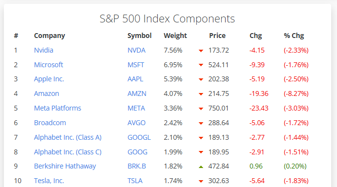
Data Sourcing: Relevant Attributes for S&P500 Components
As mentioned, the goal of this project is to predict the Probability of Default (PD) for every company currently in the S&P 500 Index. The S&P 500 is one of the most widely tracked stock market indices in the world, made up of 500 large, publicly traded companies listed on U.S. exchanges. Companies are chosen for the index based on factors like market size, liquidity, and sector representation, and the list is reviewed regularly to reflect changes in the market.
The reason I chose the S&P 500 constituents, is that getting a complete set of requisite data in order to generate the Probability of Default would be easier that it would be for mid to small-caps.
To get the list of current S&P 500 companies, I used Slickcharts, which provides an up-to-date breakdown of the index and its constituents. I simply copy-and-pasted this list into Excel, and saved as a csv file, that will allow me to load into my model to identify the companies I’ll be generating the PD for.
Data Sourcing: Company Specific Data from Yahoo Finance
Yahoo Finance remains one of the more accessible and surprisingly comprehensive sources of financial data available for free. While it may not carry the weight of institutional-grade vendors like Bloomberg or Refinitiv, it serves as a highly effective starting point for data-driven research and model development, particularly when exploring firm-level attributes for credit risk modelling. It will be the primary source of company specific data that I will use in my modelling approaches.
One of the major advantages of using Yahoo Finance is that it does not require traditional web scraping, instead, the data can be accessed programmatically through open-source libraries such as yfinance, which provide a convenient interface for retrieving historical prices, financial statements, valuation ratios, and other market-level indicators. This significantly simplifies the data acquisition process, allowing for automated collection without navigating the structure of a front-end webpage or handling changes in HTML layouts.
Accessing the Yahoo Finance API
To begin the process, I load in the 500 constituents into a “ticker_list” array, that will serve as the input into my API calls, so that Yahoo Finance will know which companies I want to return data for. I just needed to take this list, and iteratively run each of the Yahoo Finance API end points, and store the data into a dataframe for later use.
import pandas as pd
import yfinance as yf
import requests
import matplotlib.pyplot as plt
import numpy as np
import time
from fredapi import Fred
from datetime import datetime
import os
import json
from yahooquery import Ticker
from scipy.stats import norm
# Packages for unsupervised learning
from sklearn.preprocessing import StandardScaler
from sklearn.impute import SimpleImputer
from sklearn.ensemble import IsolationForest
from sklearn.neighbors import LocalOutlierFactor

start_date = "2020-07-01"
end_date = "2025-06-30"

sp500_components = pd.read_csv('S&P500Tickers.csv', skipinitialspace=True, encoding='latin1')
ticker_list = sp500_components['Ticker'].dropna().unique().tolist()

def get_latest_value(df, row_name):
    if df.empty or row_name not in df.index:
        return np.nan
    if isinstance(df.columns, pd.MultiIndex):
        df.columns = ['_'.join(map(str, col)).strip() for col in df.columns.values]
    try:
        latest_col = df.columns[0]
        val = df.loc[row_name, latest_col]
        if isinstance(val, pd.Series):
            val = val.iloc[0]
        return val
    except Exception:
        return np.nan

def fetch_data(ticker_list, start_date, end_date):
    records = []

    yf_extract = yf.download(tickers=ticker_list, start=start_date, end=end_date,
                             group_by='ticker', auto_adjust=False, threads=True, progress=True)

    for ticker in ticker_list:
        print(f"Processing {ticker} price data...")

        try:
            ticker_df = yf_extract[ticker].copy()
            if ticker_df.empty:
                print(f"Warning: no price data for {ticker}")
                continue

            # Rename so its easy to understand
            ticker_df = ticker_df.rename(columns={
                'Open': 'Open Price',
                'High': 'High Price',
                'Low': 'Low Price',
                'Close': 'Close Price',
                'Adj Close': 'Adjusted Close Price',
                'Volume': 'Volume'
            })

            price_series = ticker_df.get('Adjusted Close Price')
            if price_series is None or price_series.isna().all():
                price_series = ticker_df['Close Price']

            # Compute log returns
            log_ret = np.log(price_series).diff()
            rolling_window = 252
            sigma_E = log_ret.rolling(window=rolling_window, min_periods=rolling_window // 2).std() * np.sqrt(252)

            tk = yf.Ticker(ticker)
            info = tk.info

            # Calculate Shares Outstanding and Market Capitalisation
            shares_outstanding = info.get('sharesOutstanding', np.nan)
            market_cap = price_series * shares_outstanding

            # Financial statement information
            balance_sheet = tk.balance_sheet
            income_stmt = tk.financials
            cashflow = tk.cashflow

            # Pull financial metrics
            long_term_debt = get_latest_value(balance_sheet, 'Long Term Debt')
            short_term_debt = get_latest_value(balance_sheet, 'Short Long Term Debt')
            if pd.isna(short_term_debt):
                short_term_debt = get_latest_value(balance_sheet, 'Short Term Debt')
            total_debt = sum(filter(pd.notna, [long_term_debt, short_term_debt]))
            total_equity = get_latest_value(balance_sheet, 'Total Stockholder Equity')
            current_assets = get_latest_value(balance_sheet, 'Total Current Assets')
            current_liabilities = get_latest_value(balance_sheet, 'Total Current Liabilities')
            operating_cash_flow = get_latest_value(cashflow, 'Total Cash From Operating Activities')
            net_income = get_latest_value(income_stmt, 'Net Income')
            total_revenue = get_latest_value(income_stmt, 'Total Revenue')
            ebitda = get_latest_value(income_stmt, 'EBITDA')

            # Calculation of ratios
            debt_equity = total_debt / total_equity if total_equity else np.nan
            current_ratio = current_assets / current_liabilities if current_liabilities else np.nan
            net_income_margin = net_income / total_revenue if total_revenue else np.nan

            # Extract as many other useful attributes as possible
            extra_fields = {
                'Beta': info.get('beta'),
                'Trailing PE': info.get('trailingPE'),
                'Forward PE': info.get('forwardPE'),
                'Price to Book': info.get('priceToBook'),
                'Return on Equity (ROE)': info.get('returnOnEquity'),
                'Return on Assets (ROA)': info.get('returnOnAssets'),
                'Profit Margin': info.get('profitMargins'),
                'Gross Margin': info.get('grossMargins'),
                'Operating Margin': info.get('operatingMargins'),
                'Revenue Growth (YoY)': info.get('revenueGrowth'),
                'Earnings Growth (YoY)': info.get('earningsGrowth'),
                'Revenue per Share': info.get('revenuePerShare'),
                'Book Value per Share': info.get('bookValue'),
                'Analyst Rating Mean': info.get('recommendationMean'),
                'Free Cash Flow (Yahoo)': info.get('freeCashflow')
            }

            # Bring it all together into a single dataframe
            temp = pd.DataFrame({
                'Date': ticker_df.index,
                'Ticker': ticker,
                'Open Price': ticker_df['Open Price'],
                'High Price': ticker_df['High Price'],
                'Low Price': ticker_df['Low Price'],
                'Close Price': ticker_df['Close Price'],
                'Adjusted Close Price': ticker_df['Adjusted Close Price'],
                'Volume': ticker_df['Volume'],
                'Price Used': price_series,
                'Log Return': log_ret,
                'Equity Volatility': sigma_E,
                'Shares Outstanding': shares_outstanding,
                'Market Cap': market_cap,
                'Debt/Equity Ratio': debt_equity,
                'Current Ratio': current_ratio,
                'Net Income Margin': net_income_margin,
                'Operating Cash Flow': operating_cash_flow,
                'EBITDA': ebitda
            })

            for key, val in extra_fields.items():
                temp[key] = val

            records.append(temp.reset_index(drop=True))

        except Exception as e:
            print(f"Error processing {ticker}: {e}")

    if records:
        df_all = pd.concat(records, ignore_index=True)
        df_all = df_all.dropna(subset=['Market Cap', 'Equity Volatility'])
        df_all = df_all[['Date', 'Ticker'] + [col for col in df_all.columns if col not in ['Date', 'Ticker']]]
        df_all.reset_index(drop=True, inplace=True)
        return df_all
    else:
        return pd.DataFrame()

data = fetch_data(ticker_list, start_date, end_date)
data.head()
The data being extracted from the Yahoo Finance API end-points are detailed below:
| Date & Ticker | The trading date and the identifier for the company. These are essential for aligning time series, tracking changes over time, and linking to other data such as sector, fundamentals, or macroeconomic indicators. |
| Open / High / Low / Close / Adjusted Close | Daily price points. Adjusted Close accounts for dividends, splits, and other corporate actions, offering the truest reflection of equity value. Historical prices feed into return calculations and help assess market behavior, which is vital for both structural models and data-driven PD approaches. |
| Volume | The number of shares traded in a day. Unusual volume can signal shifting market sentiment, emerging distress, or significant events, and can serve as a predictive feature in machine learning models for default risk. |
| Price Used | The chosen price series (typically Adjusted Close) for calculating returns and deriving equity value. Consistency here ensures the inputs to volatility and option-based models are meaningful. |
| Log Return | The natural log of consecutive price ratios, representing the daily return. This is the basis for estimating realised volatility, which feeds directly into structural models like Merton and helps capture momentum or deterioration signals in machine learning models. |
| Equity Volatility | Annualised volatility derived from rolling log returns (usually over a 252 trading day window). In the Merton framework, it is a key input for inferring asset volatility and thus the likelihood of default. In statistical models, it reflects uncertainty about future performance. |
| Shares Outstanding | The total number of issued shares. Combined with price, it gives the market value of equity. Changes in this figure affect capital structure and investor perception, and therefore can influence default assessments. |
| Market Cap | Price multiplied by shares outstanding, representing the market value of equity. Serves as the equity value input in structural PD models and provides a sense of firm size and market confidence in both model types. |
| EBITDA | Earnings before interest, taxes, depreciation, and amortisation, which is a proxy for operating cash flow. High or growing EBITDA indicates stronger financial health and lower risk of default. |
| Operating Cash Flow | Cash generated from core operations. Firms with strong operating cash flow are more likely to survive downturns, even with high debt. |
| Net Income | Total earnings after expenses and taxes. Persistent losses increase the probability of financial distress and can be a leading indicator of default. |
| Profit Margin | Net income divided by revenue. Reflects operational efficiency. Low or declining margins could indicate cost pressures or pricing challenges, which are early signals of stress. |
| Current Ratio | Current assets divided by current liabilities. A liquidity measure, where ratios below 1 may indicate short-term solvency risk. |
| Debt to Equity Ratio | A leverage metric, calculated as total debt divided by shareholders’ equity. High values signal dependency on debt financing, which can elevate PD, especially in downturns. |
| Beta (5Y Monthly) | A measure of systematic risk, i.e. how volatile the stock is relative to the market. Can be used to estimate asset volatility in Merton-type models or as a risk proxy in ML approaches. |
| Analyst Recommendation Mean | A market sentiment indicator on a 1 (Strong Buy) to 5 (Sell) scale. May reflect soft signals about a firm’s outlook, which is useful when integrated with hard financial metrics. |
By automating this workflow, I was able to generate a structured dataset where each row corresponds to a specific entity and time point, with aligned variables across companies. This consistency is critical when comparing firms or training predictive models, as it ensures that input features are standardised and reliably sourced. The ability to repeatedly update the data with a single script also makes this approach well suited to ongoing analysis and production-level deployment, where fresh market inputs are essential.
Unfortunately when checking my data, it was clear that a critical element, the Debt/Equity Ratio, was entirely blank, which would make it impossible to generate the Probability of Default for the Merton model. The reason this attribute is important, is that it is a measure of financial leverage indicating how much debt a company uses to finance its assets compared to shareholders’ equity.
For large U.S. companies, like those in the S&P 500, the median D/E ratio typically falls between 0.3 and 0.7, depending on the industry. Some sectors, such as utilities and financials, tend to carry higher debt, while tech companies often have lower leverage. This range reflects the diversity of capital structures across the market.
Given the difficulty of obtaining clean debt data, I will use a proxy ratio of 0.5. It represents a moderate level of leverage near the middle of the typical range, allowing me to proceed with Merton PD calculations that would otherwise fail.
Data Sourcing: Macroeconomic Indicators from FRED API
The FRED API, maintained by the Federal Reserve Bank of St. Louis, is a well-established and freely accessible source of macroeconomic data. It offers a wide range of economic indicators that can be pulled directly into a project without needing to download files manually or set up scraping processes. This makes it particularly useful when working with models that require time series data, such as those used to estimate the probability of default.
In this case, the FRED API is used to collect a selection of indicators that are known to influence credit risk. These include standard measures such as the unemployment rate, inflation through the Consumer Price Index, interest rates, and the slope of the yield curve. Together, they offer a view of the broader economic environment in which a firm operates.
Each data point is indexed by date, which allows it to be matched against firm-level data like share price, debt levels, or volatility. This alignment is important when building a time-aware model that needs to understand how changing economic conditions might contribute to financial stress or an increased likelihood of default. Because macroeconomic variables tend to have effects that play out over time, including them helps the model identify both gradual trends and sharper shifts in credit conditions.
Accessing the FRED API
Unlike the Yahoo Finance API, I need an API key to access the FRED API, which can be generated after creating an account here.
With the key stored in my Python code, I can then run the extracts of macroeconomic data (which is monthly), that I then forward-fill to get daily data:
DATA_FILE = "macro_indicators.csv"

# Check if the file already exists
if os.path.exists(DATA_FILE):
    print("Loading existing FRED data from file...")
    macro_df = pd.read_csv(DATA_FILE, parse_dates=["Date"])
else:
    print("No existing data found. Pulling from FRED API...")

    fred = Fred(api_key=FRED_API_KEY)

    # Define extended indicators
    indicators = {
        "UNRATE": "Unemployment Rate (%)",
        "CPIAUCSL": "Consumer Price Index (CPI)",
        "FEDFUNDS": "Federal Funds Rate",
        "GS10": "10-Year Treasury Constant Maturity Rate",
        "T10Y2Y": "10Y-2Y Treasury Spread",
        "GDP": "Real Gross Domestic Product",

        # New macro/credit indicators
        "BAA10Y": "Baa Spread (Moody’s Baa - 10Y Treasury)",
        "BAMLH0A0HYM2": "High Yield Credit Spread",
        "BAMLC0A4CBBB": "BBB Corporate Bond Yield",
        "VIXCLS": "VIX Volatility Index",
        "RECPROUSM156N": "Recession Probability",
        "DGS2": "2-Year Treasury Rate",
        "M2SL": "Money Supply (M2)",
        "BUSLOANS": "C&I Loans Outstanding",
        "SLOAS": "Banks Tightening C&I Loan Standards"
    }

    start_date = "2015-01-01"
    end_date = datetime.today().strftime("%Y-%m-%d")

    macro_df = pd.DataFrame()

    for code, label in indicators.items():
        try:
            print(f"Pulling: {label}")
            series = fred.get_series(code, observation_start=start_date, observation_end=end_date)
            macro_df[label] = series
        except Exception as e:
            print(f"Failed to fetch {label} ({code}): {e}")

    macro_df = macro_df.reset_index().rename(columns={"index": "Date"})
    macro_df.fillna(method='ffill', inplace=True)

    macro_df.to_csv(DATA_FILE, index=False)
    print(f"FRED macro data saved to: {DATA_FILE}")

if 'Date' in macro_df.columns:
    macro_df['Date'] = pd.to_datetime(macro_df['Date'])
    macro_df = macro_df.set_index('Date')

all_dates = pd.date_range(start=macro_df.index.min(), end=macro_df.index.max(), freq='D')

macro_full_df = macro_df.reindex(all_dates).ffill()

macro_full_df = macro_full_df.rename_axis('Date').reset_index()

# Show sample
macro_full_df.head()
The indicators I have extracted are summarised in the table below, along with a brief explanation of how each contributes to the overall picture of risk. These variables do not replace firm-level metrics, but they do provide essential context that can strengthen a model’s ability to assess creditworthiness, particularly in periods of economic uncertainty.
| Date | The calendar date of the observation. Used to align economic indicators chronologically and enable time series analysis and correlation with market and firm-level data. |
| Unemployment Rate (%) | The percentage of the labor force that is unemployed and actively seeking employment. A key indicator of economic health and labor market conditions, which can influence credit risk and economic cycles. |
| Consumer Price Index (CPI) | Measures the average change over time in prices paid by urban consumers for a market basket of consumer goods and services. Used as a gauge of inflation, affecting real returns and monetary policy expectations. |
| Federal Funds Rate | The interest rate at which banks lend reserves to each other overnight. It reflects monetary policy stance and impacts borrowing costs, discount rates, and economic activity. |
| 10-Year Treasury Constant Maturity Rate | The yield on 10-year U.S. Treasury securities, representing long-term risk-free interest rates. Important for discounting cash flows and reflecting market expectations of growth and inflation. |
| 10Y-2Y Treasury Spread | The difference between the 10-year and 2-year Treasury yields. Often used as an indicator of economic outlook and recession risk; an inverted spread can signal impending downturns. |
| Real Gross Domestic Product (GDP) | Inflation-adjusted value of all goods and services produced in the economy. A fundamental indicator of economic growth and business cycle phase, impacting credit risk and investment decisions. |
The Merton Structural Model
The Merton model is one of the earliest and most influential approaches in credit risk modelling. Developed by Robert Merton in 1974, it offers an elegant way to estimate the Probability of Default based on the value and volatility of a firm’s assets, using concepts borrowed from option pricing theory. The key insight is to treat a company’s equity as a European call option on its assets, where the strike price corresponds to the face value of the company’s debt due at a future time, typically one year.
The model views the firm as a bundle of assets financed by debt and equity. At the debt maturity date, debt holders have the right to claim the firm’s assets up to the value of the debt. If the assets are worth less than the debt, the firm defaults. For equity holders, this situation resembles owning a call option: if the asset value exceeds the debt, equity holders receive the residual value, otherwise they lose everything.
To apply the model, we require several inputs from market data and financial statements. These include the market value of equity, which can be obtained by multiplying the number of outstanding shares by the current share price, the equity volatility estimated from historical equity returns, the face value of debt drawn from the balance sheet, the time horizon for the analysis (usually one year), and the risk-free interest rate representing the economic environment – all attributes that have been extracted in the previous sections.
Mathematically, the equity value is expressed as the value of a call option on the firm’s assets:
where E is the market equity value, V is the unobservable asset value, D is the face value of debt, r is the risk-free rate, and T is the time horizon.
The terms d1 and d2 are defined as:
with σV representing the volatility of the firm’s assets, and N(⋅) being the standard normal cumulative distribution function.
The challenge is that while equity value E and equity volatility σE are observable, the asset value V and asset volatility σV are not. The model uses a system of two nonlinear equations, linking E, σE, V, and σV, which must be solved iteratively to infer V and σV.
Once these are estimated, the model calculates the Distance to Default (DD), which measures how many standard deviations the firm’s assets are away from the default point:
The probability of default over the time horizon is then given by the probability that the asset value will fall below the debt threshold, which is the standard normal cumulative probability of minus the distance to default:
This probability quantifies the likelihood that the firm will default within the period.
Setting up the Model
Using the data I extracted primarily from Yahoo Finance, I have everything I need to calculate the Probability of Default using the Merton approach.
The attributes I need are: Market Capitalisation, Debt/Equity Ratio, Log Returns, and the 2-Year Treasury Rate.
With this information, I will perform the following calculation steps:
- Calculate the 5-year annualised equity volatility per ticker from the Log Returns: With the returns, I can estimate daily volatility (standard deviation), which is then annualised by multiplying by multiplying by the square root of 252 days (root t scaling of the number of business days in a year
- Take the most recent snapshot of data for each company
- Remove any values that aren’t valid (e.g. missing, or zero), as the model will fail without them
- Calculate the Merton model, which is to assume the equity of each ticker is a call option on it’s assets:
- Debt = Market Capitalisation * Debt/Equity Ratio
- Firm Value = Debt + Market Capitalisation
- Asset Volatility = Equity Volatility * Market Capitalisation / Firm Value
- Finally, using the formula above, calculate d1, d2 and then the Probability of Default:
final_df.columns = final_df.columns.str.strip()

#Calculate 5-year annualised equity volatility per ticker from Log Returns
#Assuming daily returns, annualise by multiplying std by sqrt(252 trading days)
volatility_per_ticker = final_df.groupby('Ticker')['Log Return'].std() * np.sqrt(252)
volatility_per_ticker = volatility_per_ticker.rename('Equity Volatility').reset_index()

#Extract the latest available data per ticker
latest_idx = final_df.groupby('Ticker')['Date'].idxmax()
latest_data = final_df.loc[latest_idx, ['Ticker', 'Market Cap', 'Debt/Equity Ratio', '2-Year Treasury Rate']]

#Merge the volatility into the latest data
latest_data = latest_data.merge(volatility_per_ticker, on='Ticker', how='left')

#Drop rows with missing critical inputs
latest_data = latest_data.dropna(subset=['Market Cap', 'Debt/Equity Ratio', 'Equity Volatility', '2-Year Treasury Rate'])

#Filter for positive numeric values
latest_data = latest_data[
    (latest_data['Market Cap'] > 0) &
    (latest_data['Debt/Equity Ratio'] > 0) &
    (latest_data['Equity Volatility'] > 0)
]

#Calculate Merton Model variables
latest_data['Debt'] = latest_data['Market Cap'] * latest_data['Debt/Equity Ratio']
latest_data['V'] = latest_data['Market Cap'] + latest_data['Debt']
latest_data['r'] = latest_data['2-Year Treasury Rate'] / 100
T = 1
latest_data['sigma_V'] = latest_data['Equity Volatility'] * latest_data['Market Cap'] / latest_data['V']
latest_data = latest_data[latest_data['sigma_V'] > 0]

#Calculate d1 and d2
latest_data['d1'] = (np.log(latest_data['V'] / latest_data['Debt']) + (latest_data['r'] + 0.5 * latest_data['sigma_V']**2) * T) / (latest_data['sigma_V'] * np.sqrt(T))
latest_data['d2'] = latest_data['d1'] - latest_data['sigma_V'] * np.sqrt(T)

#Calculate Probability of Default using cumulative normal distribution
latest_data['PD_Merton'] = norm.cdf(-latest_data['d2'])

#Final output: ticker and PD
pd_per_ticker = latest_data[['Ticker', 'PD_Merton']].reset_index(drop=True)
pd_per_ticker.to_csv('merton_pd.csv')

print(pd_per_ticker)
When most people think of the S&P 500, they think of large, stable, and dependable companies, rather than those they would expect to be at risk of default. Using this Merton model, it was clear that this is the case for the vast majority, but even within an index of corporate giants, there are a few that definitely stand out in the top ten:
| Rank | Ticker | Company | PD Merton |
|---|---|---|---|
| 1 | COIN | Coinbase Global | 5.994% |
| 2 | SMCI | Supermicro | 3.534% |
| 3 | ENPH | Enphase Energy | 1.195% |
| 4 | TTD | The Trade Desk | 1.099% |
| 5 | MRNA | Moderna | 1.041% |
| 6 | PLTR | Palantir Technologies | 1.011% |
| 7 | XYZ | Block | 0.565% |
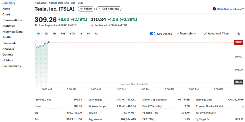
| 8 | TSLA | Tesla, Inc. | 0.539% |
| 9 | GEV | GE Vernova | 0.371% |
| 10 | NCLH | Norwegian Cruise Line Holdings | 0.332% |
Coinbase Global (COIN): 5.99% PD
The only pure crypto exchange in the index, Coinbase’s fortunes are tied directly to the highly volatile crypto markets. Bitcoin price swings, shifting regulation, and competitive threats all feed into the extreme volatility of its stock, which the model reads as heightened risk. Not surprisingly, this tops the list!
Supermicro (SMCI): 3.53% PD
A company that has ridden the wave of the AI hardware boom, but that success clearly comes with vulnerability. SMCI’s revenues are closely tied to big-ticket tech infrastructure spending, which can dry up quickly if corporate budgets tighten. The stock’s wild moves are enough to push it near the top of the list.
Enphase Energy (ENPH): 1.20% PD
The solar equipment leader is battling rising interest rates (which has hurt solar adoption) and supply chain pressures. Growth has slowed, and while the company isn’t drowning in debt, investor sentiment has cooled significantly, which has resulted in more volatile shares.
Unsupervised Anomaly Detection
Having already implemented a structural approach to estimating the Probability of Default (PD) using the Merton model, I wanted to complement it with a more flexible, data-driven methodology. While structural models are grounded in financial theory, they rely on restrictive assumptions such as constant asset volatility, simplistic capital structures, and the availability of precise inputs like the market value of debt, assumptions that are often violated in practice.
A seemingly obvious next step would be to apply a supervised machine learning model such as XGBoost to predict default or replicate PD estimates; however, supervised models suffer from an inherent limitation in this context in that they require a labelled target. When that target (PD) is itself derived from a model using similar input features, the machine learning model risks merely rediscovering the same relationships, leading to artificially high performance metrics (e.g., an R² close to 1) without offering new insight.
To avoid this issue, I decided the best approach was to implement unsupervised anomaly detection, which does not rely on a labelled target variable. These models identify unusual patterns in the data based purely on feature distributions, making them well-suited for finding hidden risks or previously unidentified outliers in financial and economic profiles for entities that may not have defaulted yet, but deviate from the norm in potentially concerning ways.
Setting up the Model
To build this, I started by combining a set of features capturing company-level fundamentals with broader macroeconomic indicators. On the company side, I included variables such as equity volatility, debt-to-equity ratio, margins, free cash flow, profitability measures like ROE and ROA, and valuation multiples including PE and price-to-book. From a market perspective, I included high-level macro factors like interest rates, CPI, and unemployment, though these were ultimately filtered out in this version due to limited variation across tickers at a single time point.
# Setting up the attributes I want to use
feature_cols = [
    'Log Return', 'Equity Volatility', 'Debt/Equity Ratio', 'Current Ratio',
    'Net Income Margin', 'Operating Cash Flow', 'EBITDA',
    'Beta', 'Trailing PE', 'Forward PE', 'Price to Book', 'Return on Equity (ROE)',
    'Return on Assets (ROA)', 'Profit Margin', 'Gross Margin',
    'Operating Margin', 'Revenue Growth (YoY)', 'Earnings Growth (YoY)',
    'Revenue per Share', 'Book Value per Share', 'Analyst Rating Mean', 'Free Cash Flow (Yahoo)'
]

# Filter for latest date data
latest_date = final_df['Date'].max()
latest_data = final_df[final_df['Date'] == latest_date].copy()

# Select features and drop rows with all NaNs in these features
X = latest_data[feature_cols]

# Impute missing values with mean
imputer = SimpleImputer(strategy='mean')
X_imputed = imputer.fit_transform(X)

scaler = StandardScaler()
X_scaled = scaler.fit_transform(X_imputed)

iso = IsolationForest(n_estimators=100, contamination=0.01, random_state=42)
iso.fit(X_scaled)
iso_scores = -iso.decision_function(X_scaled)

lof = LocalOutlierFactor(n_neighbors=20, contamination=0.01)
lof_scores = -lof.fit_predict(X_scaled)  # LOF returns -1/1, but we want scores:
lof_scores = -lof.negative_outlier_factor_

# Build results DataFrame
results = latest_data[['Ticker']].copy()
results['IsolationForest_Score'] = iso_scores
results['LOF_Score'] = lof_scores

# Show top anomalies
top_iso = results.sort_values('IsolationForest_Score', ascending=False).head(10)
top_lof = results.sort_values('LOF_Score', ascending=False).head(10)

print("Top anomalies by Isolation Forest:")
print(top_iso)

print("\nTop anomalies by LOF:")
print(top_lof)
Once the dataset was prepared, I filtered for the most recent date available and selected the relevant features. Missing values were filled using mean imputation to preserve the breadth of the dataset, and I standardised all features to have a mean of zero and standard deviation of one, a necessary step for many machine learning models that are sensitive to scale.
With the data cleaned and scaled, I applied two unsupervised anomaly detection models: Isolation Forest and Local Outlier Factor (LOF).
- Isolation Forest works by randomly partitioning the data and checking how quickly each observation is isolated; more anomalous points are easier to separate and get higher scores.
- LOF, on the other hand, calculates a local density around each observation and flags points that are much less dense than their neighbours.
In both models, higher anomaly scores suggest that the company’s financial and valuation profile is unusual compared to the rest of the dataset.
Once the models were trained, I took the anomaly scores and matched them back to company tickers. This gave me a ranked list of which firms look the most anomalous according to each model. The results were interesting.
Isolation Forest Scores:
| Rank | Ticker | Company | IsolationForest Score |
|---|---|---|---|
| 1 | MRNA | Moderna | 0.11 |
| 2 | PLTR | Palantir Technologies | 0.09 |
| 3 | NVDA | Nvidia | 0.07 |
| 4 | COIN | Coinbase Global | 0.02 |
| 5 | BA | Boeing | 0.02 |
| 6 | COF | Capital One | – |
| 7 | TTWO | Take-Two Interactive | -0.04 |
| 8 | NVR | NVR, Inc. | -0.05 |
| 9 | EQT | EQT Corporation | -0.05 |
| 10 | MSFT | Microsoft | -0.06 |
Moderna (MRNA): Isolation Forest Score: 0.11
Few companies have experienced the kind of boom-and-cool-off cycle that Moderna has. The pandemic sent revenues and profits to unprecedented heights, but the post-COVID landscape has brought volatility in earnings, shifting demand, and a race to diversify the pipeline. The model likely spotted this unusual revenue trajectory and large swings in valuation.
Palantir Technologies (PLTR): Isolation Forest Score: 0.09
Palantir has a unique mix of government contracts, AI hype, and controversial valuation debates. Its revenue growth pattern and stock behaviour differ sharply from traditional software firms. Big jumps in investor sentiment, rather than steady fundamentals, may have flagged it as an anomaly.
Mvidia (NVDA): Isolation Forest Score: 0.07
Nvidia’s meteoric rise on the back of the AI boom has made its valuation, margins, and growth rates extreme outliers. It’s a textbook case of a “positive anomaly”, the model likely picked up on revenue growth multiples and market cap expansion far beyond industry norms.
It is important to note that these aren’t necessarily “bad” outliers; sometimes they’re leaders, sometimes they’re in transition, and sometimes they’re in trouble. In all cases, the model is telling us: “This stock doesn’t behave like the others.”
Local Outlier Factor:
| Rank | Ticker | Company | LOF Score |
|---|---|---|---|
| 1 | HCA | HCA Healthcare | 11.82837978 |
| 2 | EQT | EQT Corporation | 6.993851284 |
| 3 | EXE | Expand Energy | 6.95131183 |
| 4 | MRNA | Moderna | 6.467004158 |
| 5 | NVR | NVR, Inc. | 6.185527222 |
| 6 | COF | Capital One | 4.725342762 |
| 7 | LYV | Live Nation Entertainment | 4.57762228 |
| 8 | COIN | Coinbase Global | 4.261798618 |
| 9 | BA | Boeing | 4.208917684 |
| 10 | PLTR | Palantir Technologies | 3.912753332 |
HCA Healthcare: Local Outlier Factor Score: 11.83
HCA tops the list by a huge margin, suggesting something quite unusual in its market or financial signals. Healthcare providers can be defensive, but when revenues, debt levels, or share price moves don’t line up with the sector’s norms, LOF takes notice. A mix of high leverage, strong post-COVID earnings shifts, and sector-specific policy risks could be adding to its “uniqueness.”
EQT Corporation: Local Outlier Factor Score: 6.99
America’s largest natural gas producer often rides the wild commodity price rollercoaster. With gas prices swinging dramatically in recent years and heavy capital expenditures, EQT’s profile can look erratic compared to more stable S&P names.
3. Expand Energy: Local Outlier Factor Score: 6.95
As an energy player, EXE’s metrics may be driven by project-based revenues, high gearing, and commodity sensitivity, all of which tend to generate “lumpy” financial patterns.
LOF is less about saying “this company is bad” and more about saying “this company is different.” For investors, “different” can mean risk, opportunity, or both, and the art lies in figuring out which it is.
Conclusion
While machine learning models can uncover patterns that aren’t immediately visible, the Merton model offers a different strength: clarity. Its structure ties default risk to well-understood drivers like leverage, asset volatility, and market value, making results easier to interpret and explain.
Compared with unsupervised approaches, which can be less transparent in how they reach conclusions, Merton’s framework makes the “why” behind a risk signal explicit. This clarity can be particularly useful when communicating findings to stakeholders or linking market movements back to fundamentals.
In these results, each high-PD company’s ranking can be traced to tangible factors the model captures, from volatility in emerging sectors to balance sheet pressures. That transparency remains a key reason why the Merton approach continues to be a valuable complement to modern data-driven techniques.